Calculating Karyogram Metrics

The CNV profiles can be summarized with aneuploidy and heterogeneity metrics. These are available for the full sample and per chromosome.

Given a CNV result matrix with N cells and T genomic bins, and CNV state \(c_{n,t}\) for cell \(n\) at bin \(t\), the metrics are defined as follows.

Aneuploidy

Aneuploidy measures the mean deviation from the baseline state \(b\) (default \(b = 1\)). Intuitively, it summarizes how many bins are gained or lost across the dataset.

\[A = \frac{1}{T \cdot N} \sum_{n=1}^{N} \sum_{t=1}^{T} |c_{n,t} - b|\]

Heterogeneity

Heterogeneity measures how different the CNV state is across cells for the same bin. For each bin, the frequencies of the observed CNV states are estimated as \(m_{f,t}\) and sorted in decreasing order.

\[H = \frac{1}{T \cdot N} \sum_{t=1}^{T} \sum_{f=0}^{S} f \cdot m_{f,t}\]

In practice:

• higher aneuploidy means more deviation from the baseline copy-number state

• higher heterogeneity means greater variability across cells within the sample

• both metrics are available genome-wide and on a per-chromosome basis

import matplotlib.pyplot as plt
import pandas as pd
import pyEpiAneufinder as pea
import seaborn as sns

res = pd.read_csv(
    "results_sample_data/outs/result_table.tsv.gz",
    sep="\t",
    index_col=0,
)

pea.compute_aneuploidy_across_sample(res)
pea.compute_heterogeneity_across_sample(res)

aneu_chrom = pea.compute_aneuploidy_by_chr(res)
heterogen_chrom = pea.compute_heterogeneity_by_chr(res)

plot_data = pd.DataFrame(
    {
        "chrom": aneu_chrom.columns.values,
        "aneu": aneu_chrom.iloc[0],
        "heterogen": heterogen_chrom.iloc[0],
    }
)

sns.scatterplot(x="aneu", y="heterogen", data=plot_data)

for i in range(len(plot_data)):
    plt.annotate(
        plot_data["chrom"][i],
        (plot_data["aneu"][i], plot_data["heterogen"][i]),
    )

plt.xlabel("Aneuploidy per chromosome")
plt.ylabel("Heterogeneity per chromosome")
plt.show()

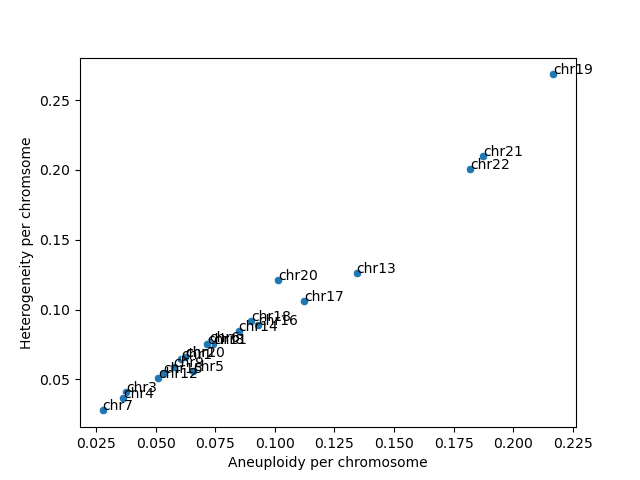
For the example data, the resulting scatter plot looks like this: